scRNA - Transfer learning for clustering single-cell RNA-Seq data
A Python framework for single-cell RNA-Seq clustering with special focus on transfer learning.
This package contains methods for generating artificial data, clustering, and transfering knowledge from a source to a target dataset.
This software package is developed by Nico Goernitz, Bettina Mieth, Marina Vidovic, and Alex Gutteridge.
Publication
The Python framework and this website are part of a publication currently under peer-review at Nature Scientific Reports. Links to the published paper and online supplementary material will be included here once available.
Abstract: In many research areas scientists are interested in clustering objects within small datasets while making use of prior knowledge from large reference datasets. We propose a method to apply the machine learning concept of transfer learning to unsupervised clustering problems and show its effectiveness in the field of single-cell RNA sequencing (scRNA-Seq). The goal of scRNA-Seq experiments is often the definition and cataloguing of cell types from the transcriptional output of individual cells. To improve the clustering of small disease- or tissue-specific datasets, for which the identification of rare cell types is often problematic, we propose a transfer learning method to utilize large and well-annotated reference datasets, such as those produced by the Human Cell Atlas. Our approach modifies the dataset of interest while incorporating key information from the larger reference dataset via Non-negative Matrix Factorization (NMF). The modified dataset is subsequently provided to a clustering algorithm. We empirically evaluate the benefits of our approach on simulated scRNA-Seq data as well as on publicly available datasets. Finally, we present results for the analysis of a recently published small dataset and find improved clustering when transferring knowledge from a large reference dataset.
News
- (2019.08) Information on the experimental results presented in our paper (under review) can be accessed in the Section “Replicating experiments”
- (2019.08) We added example application using Jupyter notebooks (cf. Section “Example application”)
- (2019.08) Added Python 3 support (scRNA no longer supports Python 2)
- (2019.08) Finalized version
- (2017.02) Added Travis-CI
- (2017.02) Added string label support
- (2017.02) Simple example available
- (2017.02) Website is up and running
- (2017.02) Wiki with detailed information (e.g. command line arguments)
- (2017.01) Please report Bugs or other inconveniences
- (2017.01) scRNA can now be conveniently installed using the pip install git+https://github.com/nicococo/scRNA.git command (see Installation for further information)
- (2017.01) Command line script available
Getting started
Installation
We assume that Python is installed and the pip command is callable from the command line. If starting from scratch, we recommend installing the Anaconda open data science platform (w/ Python 3) which comes with a bunch of most useful packages for scientific computing.
The scRNA software package can be installed using the pip install git+https://github.com/nicococo/scRNA.git command. After successful completion, three command line arguments will be available for MacOS and Linux only:
- scRNA-generate-data.sh
- scRNA-source.sh
- scRNA-target.sh
Example
Step 1: Installation with pip install git+https://github.com/nicococo/scRNA.git

Step 2: Check the scripts

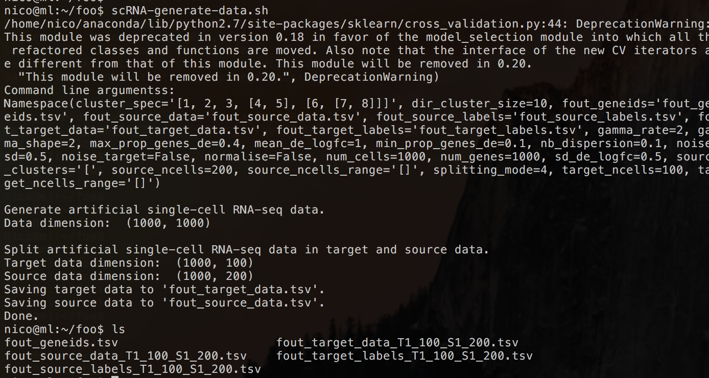
Step 3: Create directory /foo. Go to directory /foo. Generate some artificial data by simply calling the scRNA-generate-data.sh (using only default parameters).

This will result in a number of files:
- Gene ids
- Source- and target data
- Source- and target ground truth labels
Step 4: NMF of source data using the provided gene ids and source data. Ie. we want to turn off the cell- and gene-filter as well as the log transformation. You can provide source labels to be used as a starting point for NMF. If not those labels will be generated via NMF Clustering. Potential problems:
- If a ‘‘Intel MKL FATAL ERROR: Cannot load libmkl_avx.so or libmkl_def.so.’’ occurs and Anaconda open data science platform is used, then use conda install mkl first.
- Depending on the data and cluster range, this step can take time. However, you can speed up the process by tuning off the t-SNE plots using the –no-tsne command (see Wiki for further information)

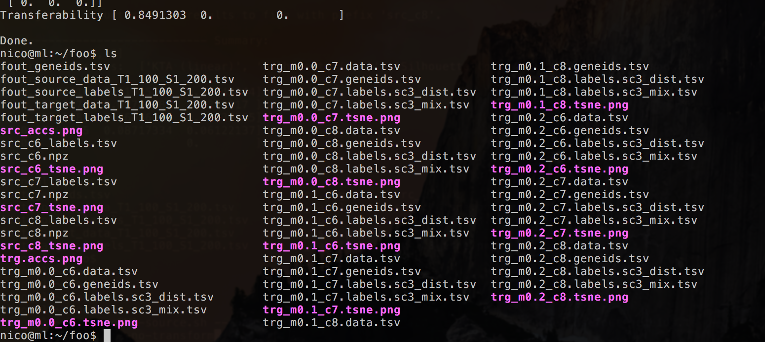
This will result in a number of files:
- t-SNE plots (.png) for every number of cluster as specified in the –cluster-range argument (default 6,7,8)
- Output source model in .npz format for every number of cluster as specified in the –cluster-range argument (default 6,7,8)
- A summarizing .png figure
- True cluster labels - either as provided from user or as generated via NMF Clustering - (and corresponding cell id) in .tsv format for every number of cluster as specified in the –cluster-range argument (default 6,7,8)
- Model cluster labels after NMF (and corresponding cell id) in .tsv format for every number of cluster as specified in the –cluster-range argument (default 6,7,8)
Step 5: Now, it is time to cluster the target data and transfer knowledge from the source model to our target data. Therefore, we need to choose a source data model which was generated in Step 4. In this example, we will pick the model with 8 cluster (src_c8.npz).
- Depending on the data, the cluster range and the mixture range, this step can take a long time. However, you can speed up the process by tuning off the t-SNE plots using the –no-tsne command (see Wiki for further information)

Which results in a number of files (for each value in the cluster range).
- Predicted cluster labels after transfer learning (and corresponding cell id) in .tsv format for every number of cluster as specified in the –cluster-range argument (default 6,7,8)
- t-SNE plots with predicted labels (.png)
- Data and gene ids in .tsv files
In addition there is a summarizing .png figure of all accs and a t-SNE plot with the real target labels, if they were provided.

Command line output shows a number of results: unsupervised and supervised (if no ground truth labels are given this will remain 0.) accuracy measures.
Example application
Using Jupyter notebooks, we showcase the main workflow as well as the abilities of the application. The main features are
- generating read-count data
- data splits using various scenarios
- source data clustering with and without accompanying labels
- augmented clustering of the target data with user defined mix-in of the source data influence.
The Jupyter notebook can be accessed under https://github.com/nicococo/scRNA/blob/master/notebooks/example.ipynb
Replicating experiments
In the course of our research (Mieth et al., see references below) we have investigated the performance of the proposed method in comparison with the most important baseline methods firstly in a simulation study on generated data, secondly on subsampled real data (Tasic et al.) and finally on two independent real datasets (Hockley et al. and Usoskin et al.). We have also shown, that batch effect removal approaches (Butler et al.) and imputation methods (Van Dijk et al.) can be used to further improve clustering results when applying our method.
- Mieth, B. et al. Clustering single-cell RNA-Seq data: An approach to transferring prior reference knowledge into datasets of small sample size. Under review at Nat. Sci. Rep. (2019)
- Tasic, B. et al. Adult mouse cortical cell taxonomy revealed by single cell transcriptomics. Nat. Neurosci. 19, 335–46 (2016).
- Hockley, J. R. F. et al. Single-cell RNAseq reveals seven classes of colonic sensory neuron. Gut. 2017–315631 (2018).
- Usoskin, D. et al. Unbiased classification of sensory neuron types by large-scale single-cell RNA sequencing. Nat. Neurosci. 18, 145–153 (2014).
- Butler, A., Hoffman, P., Smibert, P., Papalexi, E. & Satija, R. Integrating single-cell transcriptomic data across different conditions, technologies, and species. Nat. Biotechnol. 36, 411-420 (2018).
- Van Dijk, D. et al. Recovering Gene Interactions from Single-Cell Data Using Data Diffusion. Cell. 174, 716-729 (2018).
To fully reproduce the experiments of our study you can find the corresponding scripts at the following links:
- Experiments on generated datasets
- Experiments on subsampled Tasic data with labels from the original publication
- Experiments on subsampled Tasic data with NMF labels
- Experiments on Hockley data with Usoskin as source data
- Robustness experiments on Hockley data with Usoskin as source data
- Robustness experiments on Hockley data with usoskin as source data and pre-processing through Seurats batch effect removal method
- Robustness experiments on Hockley data with usoskin as source data and pre-processing through MAGIC imputation
For producing the figures of the paper go to:
For evaluating the robustness experiments producing table 1 of the paper go to:
Parameter Selection
All pre-processing parameters of the experiments presented in the paper can be found in the corresponding scripts (above) and in the online supplementary material (for the generated datasets in Supplementary Sections 2.1, for the Tasic data in Supplementary Sections 3.1 and for the Hockley and Usoskin datasets in Supplementary Sections 4.1. Details on all other parameters of the respective datasets can also be found in the scripts or in the corresponding sections of the supplementary online material (Supplementary Sections 2.2, 3.2 and 4.2, respectively).
Data availability
The datasets analyzed during the current study are available in the following GEO repositories:
- Tasic et al. (2016): https://www.ncbi.nlm.nih.gov/geo/query/acc.cgi?acc=GSE71585.
- Usoskin et al. (2014): https://www.ncbi.nlm.nih.gov/geo/query/acc.cgi?acc=GSE59739
- Hockley et al. (2018): https://www.ncbi.nlm.nih.gov/geo/query/acc.cgi?acc=GSE102962
- The command line script for simulating scRNA-Seq datasets is available at https://github.com/nicococo/scRNA/blob/master/scRNA/cmd_generate_data.py.